Activation functions

Exact moment calculations throught analytical expression for piecewise-linear activation functions

For piecewise linear activation functions such as ReLU, we can exactly compute the output moments for a Gaussian input \(Z\sim\mathcal{N}(\mu_Z,\sigma_Z^2)\). As illustrated in the figure below, this can be seen as a mixture of Gaussians where each linear segment is asociated with a probability along with moment associated with a truncated Gaussian.

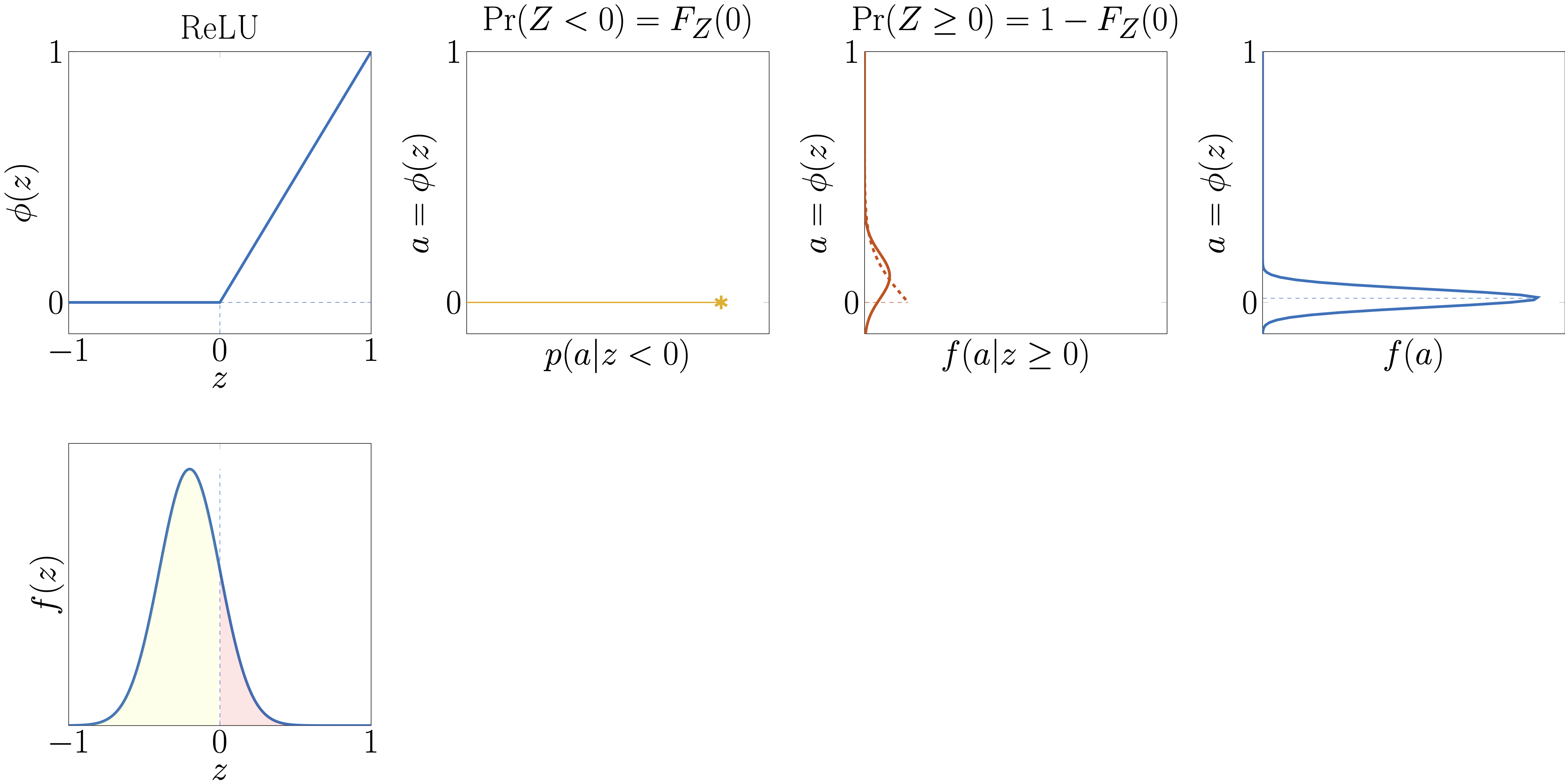
Illustration of how an input Gaussian random variable \(Z\sim\mathcal{N}(\mu_Z,\sigma_Z^2)\) is passed through a pieciwise-linear activation function such as ReLU.

The formulations for the analytical expressions for the mixture-based ReLU and Tanh presented below have been derived by Lucas Alric.

Mixture ReLU

Given a hidden unit \(z\), the pytagi.nn.activation.MixtureReLU() activation function relies on the following equations where \(\Phi(\cdot)\) denotes the standard normal CDF and \(\phi(\cdot)\) / \(\varphi(\cdot)\) denote the standard normal PDF:

\[\begin{split}\begin{aligned} a &= \phi_{\mathrm{R}}(z) = \max(0, z) \\[4pt] \mu_A &= \mu_Z \cdot \Phi\!\left(\frac{\mu_Z}{\sigma_Z}\right) + \sigma_Z \cdot \varphi\!\left(\frac{\mu_Z}{\sigma_Z}\right) \\[8pt] \sigma_A^2 &= -\mu_A^2 + 2\mu_A \mu_Z - \mu_Z \sigma_Z \, \phi\!\left(\frac{\mu_Z}{\sigma_Z}\right) + \left(\sigma_Z^2 - \mu_Z^2\right)\Phi\!\left(\frac{\mu_Z}{\sigma_Z}\right) \\[8pt] \operatorname{cov}(A,Z) &= \sigma_Z^2 \, \Phi\!\left(\frac{\mu_Z}{\sigma_Z}\right) \\[8pt] J &= \frac{\operatorname{cov}(A,Z)}{\sigma_Z^2} = \Phi\!\left(\frac{\mu_Z}{\sigma_Z}\right) \\[4pt] \operatorname{cov}(A,H) &= \rho_{ZH}\, \sigma_Z \, \sigma_H \, \Phi\!\left(\frac{\mu_Z}{\sigma_Z}\right) \end{aligned}\end{split}\]

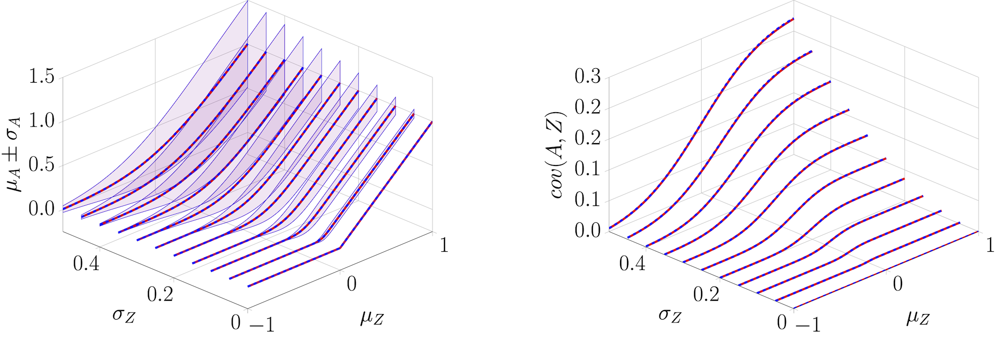
Comparison of the exact mixtureReLU (red) output moments \(\{\mu_A,\ \sigma_A,\ \operatorname{cov}(A,Z)\}\) with the theoretical values (blue) obtained through MC sampling as a function of \(\mu_Z\) and \(\sigma_Z\).

Mixture Tanh

Given a hidden unit \(z\), the pytagi.nn.activation.MixtureTanh() activation function simplifies the Tanh function by piecewise linear segments. The formulation relies on the following equations where \(\Phi(\cdot)\) denotes the standard normal CDF and \(\phi(\cdot)\) / \(\varphi(\cdot)\) denote the standard normal PDF:

\[\begin{split}\begin{aligned} a &= \phi_{\mathrm{T}}(z) = \min(\max(-1, z), 1) \\[4pt] \alpha_l &= \frac{1+\mu_Z}{\sigma_Z} \\[4pt] \alpha_u &= \frac{1-\mu_Z}{\sigma_Z} \\[8pt] \mu_A &= (\mu_Z + 1)\,\Phi(\alpha_l) + (\mu_Z - 1)\,\Phi(\alpha_u) + \sigma_Z \left( \varphi(\alpha_l) - \varphi(\alpha_u) \right) - \mu_Z \\[8pt] \sigma_A^2 &= \Phi(\alpha_l)\left(\sigma_Z^2 - \mu_Z^2 - 2\mu_Z - 1\right) \\ &\quad + \Phi(\alpha_u)\left(\sigma_Z^2 - \mu_Z^2 + 2\mu_Z - 1\right) \\ &\quad + \sigma_Z\Big(\phi(\alpha_u)(\mu_Z - 1) - \phi(\alpha_l)(\mu_Z + 1)\Big) \\ &\quad - \mu_A^2 + 2\mu_A \mu_Z + \mu_Z^2 - \sigma_Z^2 + 2 \\[8pt] \operatorname{cov}(A,Z) &= \sigma_Z^2 \Big(\Phi(\alpha_u) + \Phi(\alpha_l) - 1\Big) \\[8pt] J &= \frac{\operatorname{cov}(A,Z)}{\sigma_Z^2} = \Phi(\alpha_u) + \Phi(\alpha_l) - 1 \end{aligned}\end{split}\]

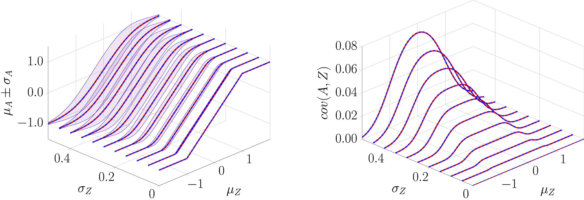
Comparison of the exact mixtureTanh (red) output moments \(\{\mu_A,\ \sigma_A,\ \operatorname{cov}(A,Z)\}\) with the theoretical values (blue) obtained through MC sampling as a function of \(\mu_Z\) and \(\sigma_Z\).

Mixture Sigmoid

The pytagi.nn.activation.MixtureSigmoid() activation function relies on a re-scaling of the MixtureTanh() activation function such that

\[a = \phi_{\mathrm{S}}(z) = \frac{\min(\max(-1, z), 1)}{2} + 0.5.\]

Thus, we can simply divide by a factor of 2 and then add 0.5 the moments obtained from mixtureTanh:

\[\begin{split}\begin{aligned} \mu_A &\leftarrow \tfrac{1}{2}\mu_A + 0.5 \\[6pt] \sigma_A^2 &\leftarrow \tfrac{1}{4}\sigma_A^2 \\[6pt] J &\leftarrow \tfrac{1}{2} J \end{aligned}\end{split}\]

Taylor-series expansion (i.e., local linearization)

When instead of relying on exact moment calculation for an activation function, we instead use the Taylor-series expansion in order to locally linearize it. In that case, the moments are obtained following the generic form

\[\begin{split}\begin{aligned} a &= \phi(z) \\[4pt] \mu_A &= \phi(\mu_Z)\\[4pt] \sigma_A^2 &= J^2\sigma_Z^2\\[4pt] J &= \left.\frac{d \phi(z)}{dz}\right|_{\mu_Z}. \end{aligned}\end{split}\]