1D toy regression heteroscedastic problem with sinusoidal data

This tutorial introduces how to use pytagi to train a regression model that is able to learn not only the signal of a sinusoidal dataset, but also the heteroscedastic aleatory uncertainty associated with it. Run it now in Google Colab.

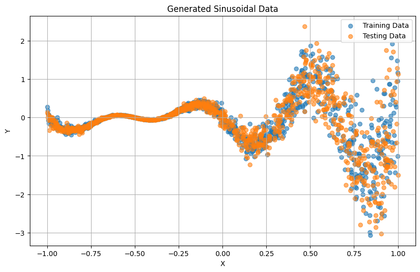
Data Generation

We define 1D toy data from a sinusoidal function. We first generate the training and testing data given \(Y=-(x+0.5)\sin(3\pi x)+ V, V \sim \mathcal{N}(0,\sigma_V^2)\) where \(\sigma_V^2=0.45(x+0.5)^2\).

# Uncomment the following lines to install the required packages if not already installed
#!pip install pytagi
#!pip install numpy
#!pip install tqdm

import numpy as np

np.random.seed(0)

def generate_data(n_samples):
    x = np.random.uniform(-1, 1, n_samples)
    v = np.random.normal(0, 0.45 * (x + 0.5) ** 2, n_samples)
    y = -(x + 0.5) * np.sin(3 * np.pi * x) + v
    return x, y

n_train_samples = 1000 # Try modifying the # of training samples to see how it affects to the epistemic uncertainty
n_test_samples = 1000

x_train, y_train = generate_data(n_train_samples)
x_test, y_test = generate_data(n_test_samples)

We can visualize the raw 1D data using matplotlib.

import matplotlib.pyplot as plt

plt.figure(figsize=(10, 6))
plt.scatter(x_train, y_train, label='Training Data', alpha=0.6)
plt.scatter(x_test, y_test, label='Testing Data', alpha=0.6)
plt.xlabel('X')
plt.ylabel('Y')
plt.title('Generated Sinusoidal Data')
plt.legend()
plt.grid(True)
plt.show()

Data Normalization

Before training a model, we need to normalize the data. Normalization is needed to bring features to a similar scale, which is key to improving the performance and training speed of TAGI.

def standardize(data, mean, std):
  return (data - mean) / std

def unstandardize(data, mean, std):
  return data * std + mean

# Manual normalization using training data statistics
mean_x = np.mean(x_train)
std_x = np.std(x_train)
x_train_scaled_manual = standardize(x_train, mean_x, std_x)
x_test_scaled_manual = standardize(x_test, mean_x, std_x)

mean_y = np.mean(y_train)
std_y = np.std(y_train)
y_train_scaled_manual = standardize(y_train, mean_y, std_y)
y_test_scaled_manual = standardize(y_test, mean_y, std_y)

Model Building

pytagi currently supports only Sequential model definition. In this case we use Linear layers and ReLU activation functions. In order to capture the aleatoric uncertainty we will need to double the number of output units in our model and add the EvenExp() layer. This layer passes through an exponential activation function the odd positions of the output layer which expected values capture the aleatoric uncertainty. Since this expected value is in the real space and our variance cannot be negative, we pass it through an exponential activation function.

from pytagi.nn import Linear, OutputUpdater, ReLU, Sequential, EvenExp

net = Sequential(
  Linear(1, 50),
  ReLU(),
  Linear(50, 50),
  ReLU(),
  Linear(50, 50),
  ReLU(),
  Linear(50, 2),
  EvenExp(), # This layer passes through an exponential activation function the odd positions of the output corresponding to
)

num_epochs = 10
batch_size = 10

out_updater = OutputUpdater(net.device)

Model Training

The training loop is simple and consist in 4 main parts:

• we do the forward pass when calling the network _, _ = net(x_batch). In this case, the output of the model will contain both aleatoric and epistemic uncertainty.

• using the out_updater.update_heteros function, where we don’t need to provide the noise cause it is already learned by the model, we update the output layer.

• we then use net.backward() and net.step() to propagate all the updated information to the parameters.

• finally we unstandardize the predictions and using the metric class, we get the MSE and log likelihood of the predictions.

In this simple tutorial we manually generate our batched data, but in general, pytagi is concived to be simple and flexible so we can rely on other libraries for the whole data processing.

from tqdm import tqdm
import pytagi.metric as metric

mses = []
pbar = tqdm(range(num_epochs), desc="Training Progress")
for epoch in pbar:
    # Create batches of the scaled training data
    num_batches = len(x_train_scaled_manual) // batch_size
    for i in range(num_batches):
        start_idx = i * batch_size
        end_idx = start_idx + batch_size
        x_batch = x_train_scaled_manual[start_idx:end_idx].reshape(-1, 1).astype(np.float32)
        y_batch = y_train_scaled_manual[start_idx:end_idx]

        # Feed forward
        m_pred, v_pred = net(x_batch)
        epistemic_variance = v_pred[::2] # Variance from Z output
        aleatoric_variance = m_pred[1::2] # Aleatoric uncertainty is expected value of odd positions
        m_pred = m_pred[::2] # We take even positions which contains Z output
        v_pred = epistemic_variance + aleatoric_variance # Add aleatoric variance to epistemic variance

        # Update output layer
        out_updater.update_heteros(
            output_states=net.output_z_buffer,
            mu_obs=y_batch,
            delta_states=net.input_delta_z_buffer,
        )

        # Feed backward
        net.backward()
        net.step()

        # Training metric
        pred = unstandardize(
            m_pred, mean_y, std_y
        )
        obs = unstandardize(y_batch, mean_y, std_y) # Unstandardize the observed batch for metric calculation
        mse = metric.mse(pred, obs)
        mses.append(mse)

    # Progress bar
    pbar.set_description(
        f"Epoch {epoch + 1}/{num_epochs}| mse: {sum(mses)/len(mses):>7.2f}",
        refresh=True,
    )

Epoch 10/10| mse:    0.23: 100%|██████████| 10/10 [00:00<00:00, 10.30it/s]

Model Testing

Similar to the training, we go through all the data and get the predictions of the model and compute the corresponding metrics.

mean_preds = []
var_preds_epistemic = []
var_preds_aleatoric = []
y_test_batches = []

num_test_batches = len(x_test_scaled_manual) // batch_size
for i in range(num_test_batches):
    start_idx = i * batch_size
    end_idx = start_idx + batch_size
    x_batch = x_test_scaled_manual[start_idx:end_idx].reshape(-1, 1).astype(np.float32)
    y_batch = y_test_scaled_manual[start_idx:end_idx].reshape(-1, 1).astype(np.float32)

    # Prediction
    m_pred_batch, v_pred_batch = net(x_batch)
    epistemic_variance = v_pred_batch[::2]
    aleatoric_variance = m_pred_batch[1::2]
    m_pred_batch = m_pred_batch[::2]
    v_pred_batch = epistemic_variance + aleatoric_variance

    # Collect predictions and original y_test values
    mean_preds.extend(m_pred_batch.flatten().tolist())
    var_preds_epistemic.extend(epistemic_variance.flatten().tolist())
    var_preds_aleatoric.extend(aleatoric_variance.flatten().tolist())
    y_test_batches.extend(y_batch.flatten().tolist())

mean_preds = np.array(mean_preds)
var_preds_epistemic = np.array(var_preds_epistemic)
var_preds_aleatoric = np.array(var_preds_aleatoric)
y_test_batches = np.array(y_test_batches)

# Add observation noise variance to the variance predictions
var_preds = var_preds_epistemic + var_preds_aleatoric
std_preds = var_preds ** 0.5

# Unstandardize the predictions and original test data for metric calculation
mean_preds_unscaled = unstandardize(mean_preds, mean_y, std_y)
std_preds_unscaled = std_preds * std_y # Unstandardize std by multiplying with original std_y
y_test_unscaled = unstandardize(y_test_batches, mean_y, std_y)


# Compute log-likelihood and MSE
mse = metric.mse(mean_preds_unscaled, y_test_unscaled)
log_lik = metric.log_likelihood(
  prediction=mean_preds_unscaled, observation=y_test_unscaled, std=std_preds_unscaled
)

print(f"Test MSE: {mse:.4f}")
print(f"Test Log-Likelihood: {log_lik:.4f}")

Test MSE: 0.1910
Test Log-Likelihood: 0.1317

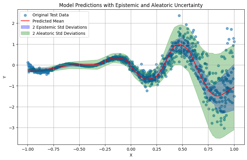
Prediction Visualization

Finally, we can visualize the predictions made by the model and distinguis the 2 uncertainties; (1) the epistemic uncertainty, corresponig to the model and (2) the aleatoric uncertainty, corresponding to the learned noise that our data has.

# Sort the test data for plotting
sorted_indices = np.argsort(x_test_scaled_manual.flatten())
x_test_sorted = x_test_scaled_manual[sorted_indices]
y_test_sorted = y_test_scaled_manual[sorted_indices]
mean_preds_sorted = mean_preds[sorted_indices]
epistemic_var_preds_sorted = var_preds_epistemic[sorted_indices]
aleatoric_var_preds_sorted = var_preds_aleatoric[sorted_indices]

# Ensure epistemic variance is non-negative
epistemic_var_preds_sorted[epistemic_var_preds_sorted < 0] = 0


epistemic_std_preds_sorted = epistemic_var_preds_sorted ** 0.5
aleatoric_std_preds_sorted = aleatoric_var_preds_sorted ** 0.5


# Unstandardize sorted data for plotting
x_test_sorted_unscaled = unstandardize(x_test_sorted, mean_x, std_x)
y_test_sorted_unscaled = unstandardize(y_test_sorted, mean_y, std_y)
mean_preds_sorted_unscaled = unstandardize(mean_preds_sorted, mean_y, std_y)
epistemic_std_preds_sorted_unscaled = epistemic_std_preds_sorted * std_y
aleatoric_std_preds_sorted_unscaled = aleatoric_std_preds_sorted * std_y


plt.figure(figsize=(10, 6))
plt.scatter(x_test_sorted_unscaled, y_test_sorted_unscaled, label='Original Test Data', alpha=0.6)
plt.plot(x_test_sorted_unscaled, mean_preds_sorted_unscaled, color='red', label='Predicted Mean')

# Plot epistemic uncertainty band
plt.fill_between(
    x_test_sorted_unscaled,
    mean_preds_sorted_unscaled - 2 * epistemic_std_preds_sorted_unscaled,
    mean_preds_sorted_unscaled + 2 * epistemic_std_preds_sorted_unscaled,
    color='blue',
    alpha=0.3,
    label='2 Epistemic Std Deviations',
)

# Plot aleatoric uncertainty band
plt.fill_between(
    x_test_sorted_unscaled,
    mean_preds_sorted_unscaled - 2 * aleatoric_std_preds_sorted_unscaled,
    mean_preds_sorted_unscaled + 2 * aleatoric_std_preds_sorted_unscaled,
    color='green',
    alpha=0.3,
    label='2 Aleatoric Std Deviations',
)


plt.xlabel('X')
plt.ylabel('Y')
plt.title('Model Predictions with Epistemic and Aleatoric Uncertainty')
plt.legend()
plt.grid(True)
plt.show()